预演：使用TensorFlow进行深度学习

2016-11-22 21:59| 发布者: joejoe0332| 查看: 822| 评论: 0|原作者: 爱不爱吃鱼, 雷神短歌, 弃天帝, 无若|来自: oschina

摘要: 本文是使用 Tensorflow 来撰写深度学习实施方案的预排，我在此只做简单地介绍。因为我不是计算机领域的专家，所以会有介绍不详尽的的地方。因此，我希望你在阅读这些代码之前，先了解相关的理论知识。 ...

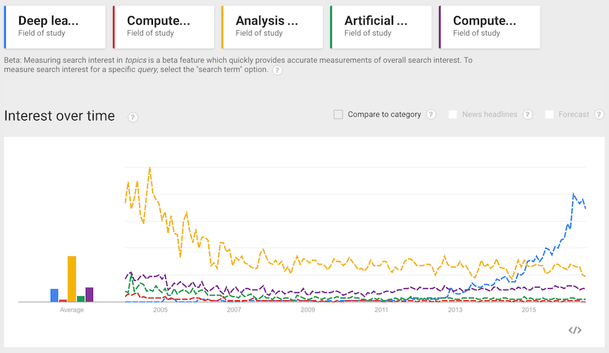
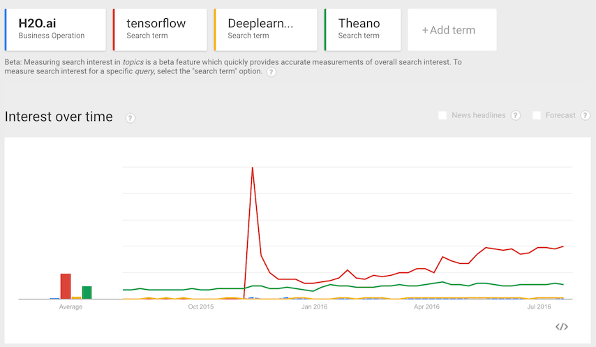
本文是使用 Tensorflow 来撰写深度学习实施方案的预排，我在此只做简单地介绍。因为我不是计算机领域的专家，所以会有介绍不详尽的的地方。因此，我希望你在阅读这些代码之前，先了解相关的理论知识。

深度学习：趋势

如今，流行语已经覆盖全球。从近些年的发展来看，“社交媒体”“物联网”加上现在的“深度学习”，都是当今流行的趋势。让我们一起来看下过去十多年间，世界计算机科学领域的研究内容。

从学术角度出发，我对研究领域做了个比较，深度学习占据第一位，紧随其后的是算法分析，计算机安全排第三，人工智能排在第四，这有点让人难以相信。排在最后的是电脑绘图，看来大家对它不怎么感兴趣。

TensorFlow: 为什么是它?

我运用深度学习的知识解决过相关的问题，但只用了不到一周的时间，如果我现在就撰写一篇学术性的文章，显然会班门弄斧。作为开发者，我想分享一下，我是如何通过深度学习编写 TensorFlow 的，这样比较实在。

我曾使用过 Theano (短暂性的)，而现在，我正在考虑使用哪款工具链比较好，也在考虑是否使用 H2O 堆，前者在世界范围内有一个很大的社区，后者则相形见绌。然而，不管怎么样，从统计图的峰值来看，谷歌的 TensorFlow 在宣传炒作上一定下了血本，也非常注重性能的提升及开发者关系的维护。显然，他们在维护从业人员关系上也花了不少心思。再顺便说一句，Theano 和 TensorFlow 都兼容 GPU。

数据集和预期结果

因为汽车评估数据集是对外公开的，所以像我这样的小白都可轻松获取。不信你也可以试试。数据集是人们就汽车使用情况进行的一项调查，它获得用户对汽车的一些反馈，如汽车价格，保养费用，车门数和容纳人数等。

样品数据如下：

1

2

3

4

5

6

vhigh,vhigh,2,2,small,low,unacc
vhigh,vhigh,2,2,small,med,unacc
vhigh,vhigh,2,2,small,high,unacc
vhigh,vhigh,2,2,med,low,unacc
vhigh,vhigh,2,2,med,med,unacc
...

我写的程序能够解析CSV格式的数据文件，然后通过反向传播生成一个多层的感知器模型，以便它能模仿人类智力，在遇到隐藏数据点时自动进行处理。

这个程序的输出应如下所示（也存在例外情况）：

Shape: (1727, 7)
 
Data types:
<class 'pandas.core.frame.DataFrame'>
RangeIndex: 1727 entries, 0 to 1726
Data columns (total 7 columns):
vhigh      1727 non-null int8
vhigh.1    1727 non-null int8
2          1727 non-null int8
2.1        1727 non-null int8
small      1727 non-null int8
low        1727 non-null int8
unacc      1727 non-null int8
dtypes: int8(7)
memory usage: 11.9 KB
 
Top 5 rows: 
   vhigh  vhigh.1  2  2.1  small  low  unacc
0      3        3  0    0      2    2      2
1      3        3  0    0      2    0      2
2      3        3  0    0      1    1      2
3      3        3  0    0      1    2      2
4      3        3  0    0      1    0      2
 
Data statistics: 
          count      mean       std  min  25%  50%  75%  max
vhigh    1727.0  1.499131  1.118098  0.0  0.5  1.0  2.0  3.0
vhigh.1  1727.0  1.499131  1.118098  0.0  0.5  1.0  2.0  3.0
2        1727.0  1.500869  1.118098  0.0  1.0  2.0  2.5  3.0
2.1      1727.0  1.000579  0.816615  0.0  0.0  1.0  2.0  2.0
small    1727.0  0.999421  0.816615  0.0  0.0  1.0  2.0  2.0
low      1727.0  1.000000  0.816970  0.0  0.0  1.0  2.0  2.0
unacc    1727.0  1.552982  0.876136  0.0  1.0  2.0  2.0  3.0
-
 
Accuracy on test dataset: 1.000000
Accuracy on training dataset: 1.000000

最后两行的输出比其他任何一项都要更具相关性。基本来说，进行的训练在规定时间内100%预测其产出等级。虽然，我们的测试目标是使得精准度最大化，但在实际操作中总会遇到障碍，最大的障碍就是我们用来训练和测试的数据的随机性。一般说来，数据输出的第一部分是统计数据，只为我们提供参考信息，你可自行忽略。

如果你仔细观察，你很快会发现，数据集在我们的输出内容里是随着数字呈现而改变的，尤其是前5行。

TensorFlow 工具链

目前 TensorFlow 的工具链还不完整，但谷歌还是在努力尝试为 TensorFlow 引入一套完整的。我认为他们这样做是对的。TensorFlow很有趣，但是它显然过于简单，对开发者的产出有所限制。因此，Google 已经开始搭建 TFLearn，又受 Scikit Learn 激发为 TensorFlow 设计了 API——这些代码编写非常有趣。还有一些其他我用过的工具，有了关于 TFLearn 和 Scikit 的学习，用这些工具能很快搭建环境。

搭建环境

首先，从这里下载，打开终端，执行以下步骤：

1

2

3

4

cd downloaded_folder
virtualenv .
source bin/activate
pip install -r requirements.txt

现在你已经拥有所有安装所需程序包，接下来，通过运行 python main.py.，你能看到一个类似我之前展现的输出。

代码预排

代码包括以下四个文件：

car-data.csv: 你就可将其理解为数据集；
requirements.txte: 此文件包含安装所需程序包列表；
main.py:代码的入口点；
categorical_dnn.py:包含所有深度学习逻辑的类别

main.py 包含的内容相对比较直白。因为它仅仅举例说明 CategoricalDNN 类，以及传递一些重要的参数。我们可以从此处了解比例，训练规模和迭代次数等。通过培训规模可知有多少比例的数据会被用来培训和其他测试。

from categorical_dnn import CategoricalDNN
 
LEARNING_RATE = 0.1
TRAINING_SIZE = 0.75 # 75%;
ITERATIONS = 1800
 
def main():
 
    dnn = CategoricalDNN('car-data.csv', TRAINING_SIZE, LEARNING_RATE,
                            ITERATIONS)
    dnn.data_insights()
    dnn.train()
 
if __name__ == "__main__":
    main()

CategoricalDNN 类假定调用程序没有关于数据的线索，这一点很关键，因为它表面了类别本身是否能够从数据中提取内容，对自身进行处理和升级。不用说，这样更有利于数据分类。

无条件DNN

我们先查看一下这个类中会用到的包：

1

2

3

4

5

6

7

import pandas as pd
import tensorflow as tf
import tensorflow.contrib.learn as tflearn
from sklearn import metrics
from sklearn.cross_validation import train_test_split
import os.path
import numpy as np

互补的内联注释能让代码更通俗易懂，而我们讨论的重点是其调用的顺序。

预处理数据

首先，_load_csvis （应该）是一个私有方法，使用 pandas 加载 CSV 到内存。然后继续计数数据集包含的列的数目。假设最后一列包含 label 或 class 信息，对应的数据集则需要被预演。

def _load_csv(self):
 
    # Loading CSV into the system using Pandas
    self._input_map = []
    self._raw_data = pd.read_csv(self._file_name, sep=',', 
                                    skipinitialspace=True)
    self._datadim = len(self._raw_data.columns)
 
    # Find uniques in the last column aka. `label` or `class`
    self._classes = self._raw_data[
                        self._raw_data.columns[self._datadim - 1]
                    ].unique()
 
    # Create a map of all unique values by columns
    for i in range(self._datadim):
        self._raw_data[self._raw_data.columns[i]] = \
            self._convert_categorical_nominal(self._raw_data, i)

最后一列包含了唯一的类，它是设计分类器的一个重要度量标准，这里再次用到了 pandas 。最后，所有的列都被循环，所有字符串都会被转换成各自的分类值以供我们的分类器处理。实际上， pandas 技巧完美地做到了 heavy-lifting 。

混合和分解

现在将数据集随机化，并分解成之前在 TRAINING_SIZE 中定义的比率。

def _shuffle_split(self):
    self._raw_data.iloc[np.random.permutation(len(self._raw_data))]
    self._testdata, self._traindata = train_test_split(
                        self._raw_data, test_size=self._training_size)
 
    # TF Learn / TensorFlow only takes int32 / int64 at the moment 
    # as oppose to int8
    self._train_label = [int(row) for row in self._traindata[
                            self._raw_data.columns[self._datadim - 1]]]
    self._test_label = [int(row) for row in self._testdata[
                            self._raw_data.columns[self._datadim - 1]]]
    self._traindata = self._traindata.ix[:, range(self._datadim - 1)]
    self._testdata = self._testdata.ix[:, range(self._datadim - 1)]

因为分类器只能使用 int32 / int64 工作，因此，我们需要转换预演和测试标签。这样也能确保标签最终不会被送入分类器，但它们在最后两行会被过滤掉。

培训模式和性能测试

现在我们已经完成预演前的所有准备工作，下一步就是设计网络。隐藏层只要合理，并能产出更好的结果，怎么安排都可以。但是根据我们的观察，以下的设计最为合适。当然还存在许多其他的优化方案，但在此我不做过多讨论。

def train(self):
 
    # The rule: my own rule aka. own intuition
    hidden_Layers = [self._datadim - 1,
                        ((self._datadim - 1) + len(self._classes)) / 2,
                        len(self._classes)]
 
    classifier = tflearn.DNNClassifier(hidden_units=hidden_Layers,
                                        n_classes=len(self._classes),
                                        activation_fn=tf.nn.relu)
 
    classifier.learning_rate = self._learning_rate
    classifier.fit(self._traindata, self._train_label, steps=self._iterations)

我将 ReLU 作为激活函数，可以按要求进行 tanh,sigmoid,softmax 等。既然模型已经设定好了，现在我们开始测试它的性能：

1

2

3

4

5

6

score = metrics.accuracy_score(self._test_label, 
                            classifier.predict(self._testdata))
print 'Accuracy on test dataset: %f' % score
score = metrics.accuracy_score(self._train_label, 
                            classifier.predict(self._traindata))
print 'Accuracy on training dataset: %f' % score

我们还是使用了 Scikit 来测试模型的准确度。